An Introduction to joker

Ioannis Oikonomidis

2025-04-25

The joker package provides a comprehensive set of features for probabilities and mathematical statistics. It extends the range of available distribution families and facilitates the computation of key parametric quantities, such as moments and information-theoretic measures. The main focus of the package is parameter estimation through maximum likelihood and moment-based methods under an intuitive and efficient coding framework.

Introduction

Package joker is designed to cover a broad collection of distribution families, extending the functionalities of the stats package to support new families, parametric quantity computation and parameter estimation. All package features are available both in a stats-like syntax for entry-level users, and in an S4 object-oriented programming system for more experienced ones.

The joker S4 Distribution System

Probability Distributions

In the joker OOP system, each distribution has a respective S4 class. The following table shows the distributions available in the package, along with their class names. All of them are subclasses of the Distribution S4 class.

library(knitr)

kable(
  data.frame(
    Distribution = c("Bernoulli", "Beta", "Binomial", "Categorical", "Cauchy",
                     "Chi-Square", "Dirichlet", "Fisher", "Gamma", "Geometric"),
    Class_Name = c("Bern", "Beta", "Binom", "Cat", "Cauchy", "Chisq", "Dir",
                   "Fisher", "Gam", "Geom"),
    Distribution2 = c("Laplace", "Log-Normal", "Multivariate Gamma",
                      "Multinomial", "Negative Binomial", "Normal", "Poisson",
                      "Student", "Uniform", "Weibull"),
    Class_Name2 = c("Laplace", "Lnorm", "Multigam", "Multinom", "Nbinom",
                    "Norm", "Pois", "Stud", "Unif", "Weib")
  ),
  col.names = c("Distribution", "Class Name", "Distribution", "Class Name"),
  caption = "Overview of the distributions implemented in the `joker` package, 
  along with their respective class names."
)

Overview of the distributions implemented in the joker package, along with their respective class names.

Distribution	Class Name	Distribution	Class Name
Bernoulli	Bern	Laplace	Laplace
Beta	Beta	Log-Normal	Lnorm
Binomial	Binom	Multivariate Gamma	Multigam
Categorical	Cat	Multinomial	Multinom
Cauchy	Cauchy	Negative Binomial	Nbinom
Chi-Square	Chisq	Normal	Norm
Dirichlet	Dir	Poisson	Pois
Fisher	Fisher	Student	Stud
Gamma	Gam	Uniform	Unif
Geometric	Geom	Weibull	Weib

Defining an object from the desired distribution class is straightforward, as seen in the following example. The parameter names, which are generally identical to the ones defined in the stats package, can be omitted.

shape1 <- 1 
shape2 <- 2
D <- Beta(shape1, shape2)

Having defined the distribution object D, the d()-p()-q()-r() functions can be used, as shown in the following example, comparing against the stats syntax.

d(D, 0.5)
> [1] 1
dbeta(0.5, shape1, shape2)
> [1] 1

p(D, 0.5)
> [1] 0.75
pbeta(0.5, shape1, shape2)
> [1] 0.75

qn(D, 0.75)
> [1] 0.5
qbeta(0.75, shape1, shape2)
> [1] 0.5

r(D, 2)
> [1] 0.2494058 0.3353119
rbeta(2, shape1, shape2)
> [1] 0.15414668 0.06689389

Alternatively, if only the distribution argument is supplied, the methods behave as functionals (i.e. they return a function). This behavior offers enhanced functionality such as:

F1 <- p(D)
F1(0.5)
> [1] 0.75

Technical Detail: The quantile function is called qn() rather than the more intuitive q(). The reason behind this choice lies in the RStudio IDE (Integrated Development Environment), which overrides the method selection process of the base function q() used to quit an R session, i.e. a function named q() always ends the session. In order to avoid this unpleasant behavior, the name qn() was chosen instead.

Parametric Quantities of Interest

The joker package contains a set of methods that calculate the theoretical moments (expectation, variance and standard deviation, skewness, excess kurtosis) and other important parametric functions (median, mode, entropy, Fisher information) of a distribution. Alternatively, the moments() function automatically finds the available methods for a given distribution and returns all of the results in a list.

mean(D)
> [1] 0.3333333
median(D)
> [1] 0.2928932
mode(D)
> [1] 0
var(D)
> [1] 0.05555556
sd(D)
> [1] 0.2357023
skew(D)
> [1] 0.5656854
kurt(D)
> [1] 0.2333333
entro(D)
> [1] -0.1931472
finf(D)
>            shape1     shape2
> shape1  1.2500000 -0.3949341
> shape2 -0.3949341  0.2500000

Technical Detail: Only the function-distribution combinations that are theoretically defined are available; for example, while var() is available for all distributions, sd() is available only for the univariate ones. In case the result is not unique, a predetermined value is returned with a warning. The following example illustrates this in the case of $\mathcal{B}(1, 1)$, i.e. a uniform distribution for which every value in the $[0, 1]$ interval is a mode.

mode(Beta(1, 1))
> Warning in mode(Beta(1, 1)): In Beta(1, 1), all elements in the [0, 1] interval are modes. 0.5
>             is returned by default.
> [1] 0.5

Parameter Estimation

The joker package includes a number of options when it comes to parameter estimation. In order to illustrate these alternatives, a random sample is generated from the Beta distribution.

set.seed(1)
shape1 <- 1
shape2 <- 2
D <- Beta(shape1, shape2)
x <- r(D, 100)

Estimation Methods

The package covers three major estimation methods: maximum likelihood estimation (MLE), moment estimation (ME), and score-adjusted moment estimation (SAME).

In order to perform parameter estimation, a new e<name>() member is added to the d()-p()-q()-r() family, following the standard stats name convention. These e<name>() functions take two arguments, the observations x (an atomic vector for univariate or a matrix for multivariate distributions) and the type of estimation method to use.

ebeta(x, type = "mle")
> $shape1
> [1] 1.066968
> 
> $shape2
> [1] 2.466715
ebeta(x, type = "me")
> $shape1
> [1] 1.074511
> 
> $shape2
> [1] 2.469756
ebeta(x, type = "same")
> $shape1
> [1] 1.067768
> 
> $shape2
> [1] 2.454257

A general function called e() is also implemented, covering all distributions and estimators.

e(D, x, type = "mle")
> $shape1
> [1] 1.066968
> 
> $shape2
> [1] 2.466715

Dominant estimation methods such as the mle(), me(), and same() are also available as S4 generics.

mle(D, x)
> $shape1
> [1] 1.066968
> 
> $shape2
> [1] 2.466715
me(D, x)
> $shape1
> [1] 1.074511
> 
> $shape2
> [1] 2.469756
same(D, x)
> $shape1
> [1] 1.067768
> 
> $shape2
> [1] 2.454257

Technical Detail: It is important to note that the S4 methods also accept a character for the distribution. The name should be the same as the S4 distribution generator, case ignored.

mle("beta", x)
mle("bEtA", x)
e("Beta", x, type = "mle")

Log-likelihood

Likewise, log-likelihood functions are available in two versions, the distribution specific one, e.g. llbeta(), and the ll() S4 generic one.

llbeta(x, shape1, shape2)
> [1] 26.56269
ll(D, x)
> [1] 26.56269

In some distribution families like beta and gamma, the MLE cannot be explicitly derived and numerical optimization algorithms have to be employed. Even in good scenarios, with plenty of observations and a smooth optimization function, numerical algorithms should not be viewed as panacea, and extra care should be taken to ensure a fast and right convergence if possible. Two important steps are taken in joker in this direction:

An illustrative example for the Beta distribution is shown below. Let $f$ denote the probability density function of $X\sim\mathcal{B}(\alpha,\beta)$:

$$f(x; \alpha, \beta) = \frac{\Gamma(\alpha + \beta)}{\Gamma(\alpha) \Gamma(\beta)}x^{\alpha-1} (1 - x)^{\beta-1}, \quad 0 < x < 1,$$

where $\Gamma$ is the Gamma function. Then, the log-likelihood function, divided by the sample size $n$, takes the form:

$$\ell(\alpha, \beta) = (\alpha - 1) \overline{\log X} + (\beta - 1) \overline{\log (1 - X)} - \log \Gamma(\alpha) - \log \Gamma(\beta) + \log \Gamma(\alpha + \beta).$$

The score equation for $\alpha$ is:

$$\frac{\partial \ell}{\partial \alpha}(\alpha, \beta) = \overline{\log X} - \psi(\alpha) + \psi(\alpha + \beta) = 0.$$

The score equation for $\beta$ is:

$$\frac{\partial \ell}{\partial \beta}(\alpha, \beta) = \overline{\log (1 - X)} - \psi(\beta) + \psi(\alpha + \beta) = 0.$$

These two nonlinear equations must be solved numerically. However, instead of solving the above two-dimensional problem, one can see that by denoting $c := \alpha + \beta$, the two score equations can be rewritten as:

$$\alpha = \psi^{-1}\left[\psi(c) + \overline{\log X}\right] \quad \beta = \psi^{-1}\left[\psi(c) + \overline{\log (1-X)}\right],$$

i.e. restricted to the score equation system solution space, both parameters can be expressed as a function of their sum $c$, and therefore the log-likelihood function can be optimized with respect to $c$:

$$\ell^\star(c) = \left[\alpha(c) - 1\right] \overline{\log X} + \left[\beta(c) - 1\right] \overline{\log (1 - X)} - \log \Gamma\left[\alpha(c)\right] - \log \Gamma\left[\beta(c)\right] + \log \Gamma(c).$$

Technical Detail: It would perhaps be more intuitive to use the score equations to express $\alpha$ as a function of $\beta$ or vice versa. However, the above method can be directly generalized to the Dirichlet case and reduce the initial $k$-dimensional problem to a unidimensional one. The same technique can be utilized for the gamma and multivariate gamma distribution families, also reducing the dimension to unity, from $2$ and $k+1$ respectively.

In joker, the resulting function that is inserted in the optimization algorithm is called lloptim(), and is not to be confused with the actual log-likelihood function ll(). The corresponding derivative is called dlloptim(). Therefore, whenever numerical computation of the MLE is required, joker calls the optim() function with the following arguments:

• lloptim(), an efficient function to be optimized,
• dlloptim(), its analytically-computed derivate,
• an initialization point (numeric) or the method to use to provide one (character, e.g. "me")
• an optimization algorithm. By default, the L-BFGS-U is used, with lower and upper limits defined at or near the parameter space boundary.

Asymptotic Variance - Covariance Matrix

The asymptotic variance (or variance - covariance matrix for multidimensional parameters) of the estimators are also covered in the package by the v<name>() functions.

vbeta(shape1, shape2, type = "mle")
>          shape1   shape2
> shape1 1.597168 2.523104
> shape2 2.523104 7.985838
vbeta(shape1, shape2, type = "me")
>        shape1 shape2
> shape1    2.1    3.3
> shape2    3.3    9.3
vbeta(shape1, shape2, type = "same")
>          shape1   shape2
> shape1 1.644934 2.539868
> shape2 2.539868 8.079736

As with point estimation, the implementation is twofold, and the general function v() covers all distributions and estimators.

avar(D, type = "mle")
avar_mle(D)
avar_me(D)
avar_same(D)

Estimation Metrics and Comparison

The different estimators of a parameter can be compared based on both finite sample and asymptotic properties. The package includes two functions named small_metrics() and large_metrics() , where small and large refers to the small sample and large sample terms that are often used for the two cases. The former estimates the bias, variance and root mean square error (RMSE) of the estimator with Monte Carlo simulations, while the latter calculates the asymptotic variance - covariance matrix (as derived by the v() functions). The resulting data frames can be plotted with the plot() function.

To illustrate the function’s design, consider the following example from the beta distribution: We are interested in calculating the metrics (bias, variance, and RMSE) of the $\alpha$ parameter estimators (MLE, ME, and SAME), for sample sizes 20 and 50. Specifically, we want to illustrate how these metrics change for $\alpha\in[1,5]$, and $\beta=2$ (constant). The following code can do that:

D <- Beta(1, 2)

prm <- list(name = "shape1",
            val = seq(1, 5, by = 0.5))

x <- small_metrics(D, prm,
             obs = c(20, 50),
             est = c("mle", "same", "me"),
             sam = 1e3,
             seed = 1)

head(x@df)
>   Parameter Observations Estimator Metric     Value
> 1       1.0           20       mle   Bias 0.1322510
> 2       1.5           20       mle   Bias 0.2486026
> 3       2.0           20       mle   Bias 0.3276922
> 4       2.5           20       mle   Bias 0.5215973
> 5       3.0           20       mle   Bias 0.5517199
> 6       3.5           20       mle   Bias 0.5381523

The small_metrics() function takes the following arguments:

• D, the distribution object of interest,
• prm, a list that specifies how the shape1 parameter values should change,
• obs, a numeric vector holding the sample sizes,
• est, a character vector specifying the estimators under comparison,
• sam, the Monte Carlo sample size to use for the metrics estimation,
• seed, a seed to be passed to set.seed() for replicability.

The resulting data frame can be passed to plot() to see the results. The package’s plot() methods depend on ggplot2 to provide highly-customizable graphs.

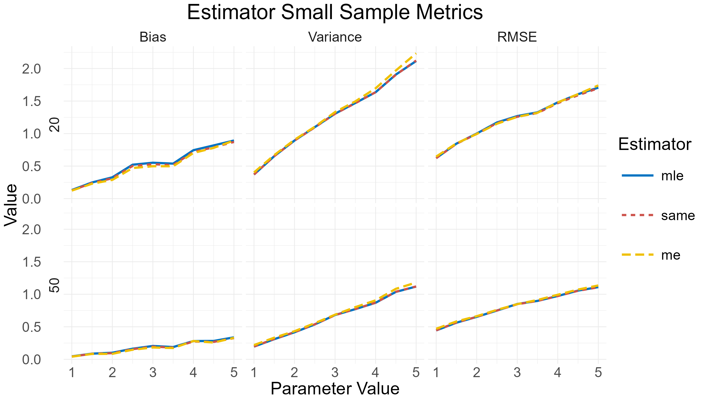
Small-sample metrics comparison for MLE, ME, and SAME of the beta distribution shape1 parameter.

Note that in some distribution families the parameter is a vector, as is the case with the Dirichlet distribution (a multivariate generalization of beta), which holds a single parameter vector alpha. In these cases, the prm list can include a third element, pos, specifying which parameter of the vector should change:

D <- Dir(alpha = 1:4)

prm <- list(name = "alpha",
            pos = 1,
            val = seq(1, 5, by = 0.5))

x <- small_metrics(D, prm,
                   obs = c(20, 50),
                   est = c("mle", "same", "me"),
                   sam = 1e3,
                   seed = 1)

class(x)
> [1] "SmallMetrics"
> attr(,"package")
> [1] "joker"
head(x@df)
>   Parameter Observations Estimator Metric      Value
> 1       1.0           20       mle   Bias 0.07759434
> 2       1.5           20       mle   Bias 0.11916042
> 3       2.0           20       mle   Bias 0.17488071
> 4       2.5           20       mle   Bias 0.20523185
> 5       3.0           20       mle   Bias 0.32907679
> 6       3.5           20       mle   Bias 0.32915767

The large_metrics() function design is almost identical, except that no obs, sam, and seed arguments are needed here. The following example illustrates the large sample metrics for the beta distribution shape $\alpha$ estimators. Again, the resulting data frame can be passed to plot().

D <- Beta(1, 2)

prm <- list(name = "shape1",
            val = seq(1, 5, by = 0.1))

x <- large_metrics(D, prm,
                   est = c("mle", "same", "me"))

class(x)
> [1] "LargeMetrics"
> attr(,"package")
> [1] "joker"
head(x@df)
>      Row    Col Parameter Estimator    Value
> 1 shape1 shape1       1.0       mle 1.597168
> 2 shape2 shape1       1.0       mle 2.523104
> 3 shape1 shape2       1.0       mle 2.523104
> 4 shape2 shape2       1.0       mle 7.985838
> 5 shape1 shape1       1.1       mle 1.969699
> 6 shape2 shape1       1.1       mle 2.826906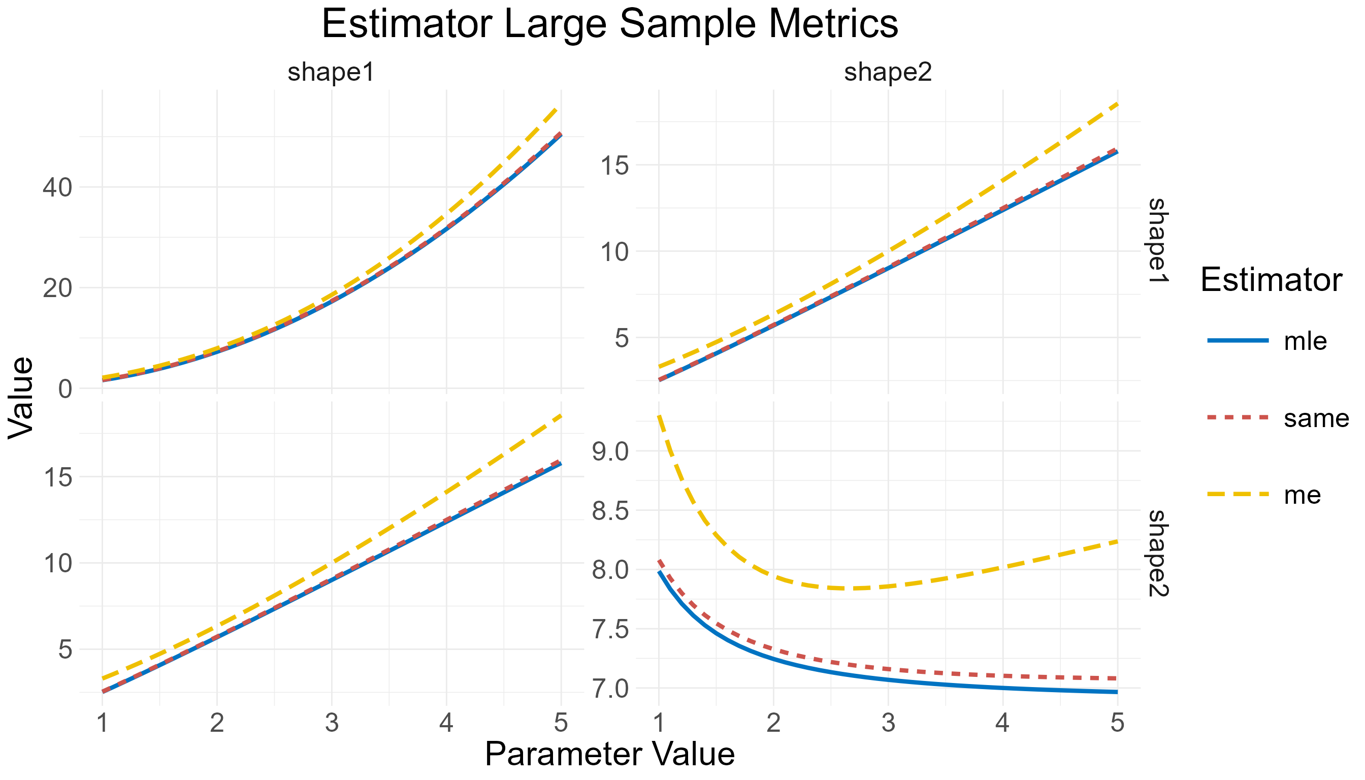

Large-sample metrics comparison for MLE, ME, and SAME of the beta distribution shape1 parameter.

Documentation and Testing

Comprehensive and clear documentation should be a central focus of every package. In joker, all functions are extensively documented, providing detailed descriptions of arguments, return values, and underlying behavior. Examples are always included to illustrate typical usage and edge cases, making it easier for users to quickly understand and apply the functions in their workflows. In addition to the function-level documentation, the package includes a thorough vignette that offers a broader overview of its functionality, demonstrates common use cases, and provides guidance on integrating the package into larger analysis pipelines, as well as information on how to expand its functionalities. This layered approach to documentation ensures that users at all levels—from new adopters to experienced developers—can make full and effective use of the package.

The joker package places a strong emphasis on rigorous testing and quality assurance. Automated testing is implemented using the testthat package, with a comprehensive suite of over 1,000 individual tests covering all core functionality. These tests ensure that all features behave as expected, edge cases are handled appropriately, and any regressions are quickly detected. Test coverage, as measured by the covr package, exceeds 90%, reflecting a thorough approach to exercising the codebase and providing a high level of confidence in the package’s reliability.

To maintain consistent code quality and immediate feedback on changes, continuous integration (CI) is set up via GitHub and CircleCI. Every pull request and push to the repository triggers a full build and test cycle, ensuring that new contributions meet the package’s standards before they are merged. This automated workflow helps to detect issues early, streamlines collaboration, and supports a development process that prioritizes stability and reproducibility.

In addition to automated testing and CI, the package complies with broader community standards and best practices. It has been validated using rOpenSci’s pkgcheck package, which ensures adherence to guidelines for documentation, code structure, and usability. Further quality assurance is provided through autotest, which automatically generates tests to explore unexpected code behaviors, and srr (Statistical Software Review), which ensures compliance with best practices specific to statistical software. Together, these tools and processes help ensure the package remains robust, maintainable, and trustworthy for users.

Defining New Classes and Methods

Of course, it is possible to be interested in a distribution family not included in the package. It is straightforward for users to define their own S4 class and methods. Since this paper is addressed to both novice and experienced R users, the beta distribution paradigm is explained in detail below:

Defining the Class

The setClass() function defines a new S4 class, i.e. the distribution of interest. The slots argument defines the parameters and their respective class (usually numeric, but it can also be a matrix in distributions like the multivariate normal and the Wishart). The optional argument prototype can be used to define the default parameter values in case they are not specified by the user.

setClass("Beta",
  contains = "Distribution",
  slots = c(shape1 = "numeric", shape2 = "numeric"),
  prototype = list(shape1 = 1, shape2 = 1))

Defining a Generator

Now that the class is defined, one can type D <- new("Beta", shape1 = shape1, shape2 = shape2) to create a new object of class Beta. However, this is not so intuitive, and a wrapper function with the class name can be used instead. This function, often called a generator, can be used to simply code D <- Beta(1, 2) and define a new object from the $\mathcal{B}(1,2)$ distribution. The parameter slots can be accessed with the @ sign, as shown below.

Beta <- function(shape1 = 1, shape2 = 1) {
  new("Beta", shape1 = shape1, shape2 = shape2)
}

D <- Beta(1, 2)
D@shape1
D@shape2

Defining Validity Checks

This step is optional but rather essential. So far, a user could type D <- Beta(-1, 2) without any errors, even though the beta parameters are defined in $\mathbb{R}_{+}$. To prevent such behaviors (that will probably end in bugs further down the road), the developer is advised to create a setValidity() function, including all the necessary restrictions posed by the parameter space.

setValidity("Beta", function(object) {
  if(length(object@shape1) != 1) {
    stop("shape1 has to be a numeric of length 1")
  }
  if(object@shape1 <= 0) {
    stop("shape1 has to be positive")
  }
  if(length(object@shape2) != 1) {
    stop("shape2 has to be a numeric of length 1")
  }
  if(object@shape2 <= 0) {
    stop("shape2 has to be positive")
  }
  TRUE
})

Defining the Class Methods

Now that everything is set, it is time to define methods for the new class. Creating functions and S4 methods in R are two very similar processes, except the latter wraps the function in setMethod() and specifies a signature class, as shown below. The package source code can be used to easily define all methods of interest for the new distribution class.

# probability density function
setMethod("d", signature = c(distr = "Beta", x = "numeric"),
          function(distr, x) {
            dbeta(x, shape1 = distr@shape1, shape2 = distr@shape2)
          })

# (theoretical) expectation
setMethod("mean",
          signature  = c(x = "Beta"),
          definition = function(x) {

  x@shape1 / (x@shape1 + x@shape2)

})

# moment estimator
setMethod("me",
          signature  = c(distr = "Beta", x = "numeric"),
          definition = function(distr, x) {

  m  <- mean(x)
  m2 <- mean(x ^ 2)
  d  <- (m - m2) / (m2 - m ^ 2)

  c(shape1 = d * m, shape2 = d * (1 - m))

})